Lava Lamp Made with Blender Geometry Nodes

Trigger warning: This article is as math heavy as it is nice to look at, but graphics are a passion of mine.

Project Scope

#

Blender’s metaballs are notoriously limited when used with Geometry Nodes (or at least, that was true at the time of development. It’s hard to keep the pace with Blender’s fast progress). We were warned about this by our professor, and thus I took it as a personal challenge of mine to come up with something that resembled metaballs as much as possible.

As you might have guessed from my website’s theming, I am a bit retro and I like lava lamps. So the project’s requirements basically materialized on their own: I wanted to make the moving wax inside a lava lamp without relying on Blender’s normal metaball objects.

The visual requirement is simple enough to describe: several rounded blobs should be able to move independently, join together when they get close, form the characteristic necks and morphs between them, and separate again as they move away.

Actually building that behavior from normal meshes is… less pleasant. Boolean operations are excessive for something this fluid, and simply intersecting spheres gives you intersecting spheres rather than a continuous surface.

This made the project a good excuse to work with Signed Distance Functions, or SDFs, inside Geometry Nodes. A signed distance function gives me a value for any position in space; evaluating it throughout a volume gives me the corresponding signed distance field.

I promise that’s about as pedantic as I’m going to get about the terminology.

Instead of treating each blob as visible geometry, I treat it as a mathematical field. The final wax surface is the zero crossing of the combination of all those fields.

That also means the animation can happen one level below the actual mesh. I only have to move a small set of control points. The SDF and final mesh react to those positions automagically.

An excellent primer on Signed Distance Functions, which will then lead you to Signed Distance Fields, is CGMatter’s video on the topic:

Starting With a Sphere SDF

#

The most basic building block is the SDF of a sphere.

For a point \(p\), sphere center \(c\), and radius \(r\):

$$ \Large d(p)=∥p−c∥−r $$

The result has a useful interpretation:

• \(d < 0\) means the point is inside the sphere
• \(d = 0\) is the sphere surface
• \(d > 0\) means the point is outside the sphere

In Geometry Nodes this becomes a very small SDF Sphere group.

The node does just what the mathematical formula says on the tin: it takes the current Position, subtracts the sphere Center, calculates the vector length, and subtracts the radius.

The important thing to note here is that there is no sphere mesh involved. Just fields, parameters and numbers. The wax blob does not actually exist as geometry yet, which feels a little fraudulent, but it will eventually.

Joining SDFs Without Hard Intersections

#

Let’s start with just two spheres, keeping it simple. Two sphere SDFs can be combined using a simple minimum:

\[ \Large d = \min(d_1,d_2) \]

That represents the union of the two shapes, but it keeps a sharp transition where the two fields meet. For lava wax I wanted the opposite. The interesting part is the soft bridge that appears as two blobs approach each other.

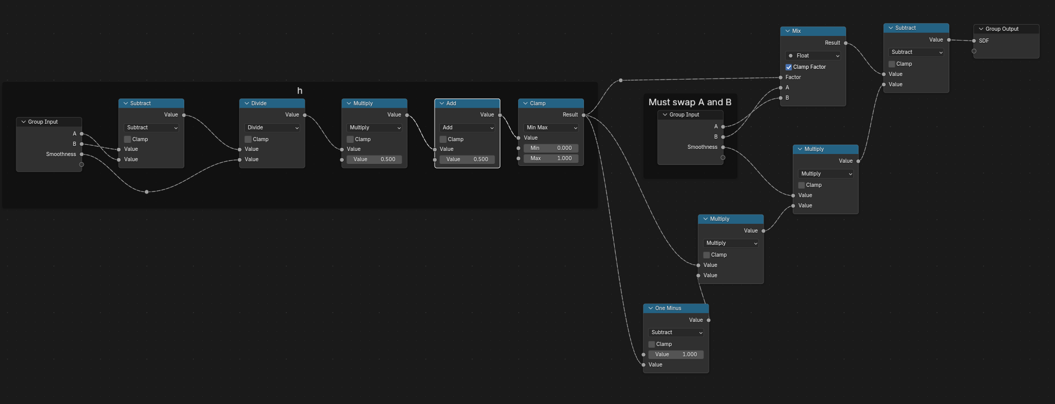
For that I made an SDF Smooth Union group based on a smooth minimum, a well known trick that conveniently does most of the visually interesting work for us.

The interpolation factor \(h\) is:

\[ \Large h = \operatorname{clamp} \left( 0.5 + 0.5\dfrac{b-a}{k}, 0, 1 \right) \]

and the resulting field \(d\) is:

\[ \Large d = \operatorname{mix}(b,a,h) - kh(1-h) \]

where \(k\) controls the blending distance.

Visually, this is one of the most important parameters in the entire setup. A low value keeps the blobs almost independent. Increasing it causes nearby blobs to pull into each other and form the soft, stretched connections that make the result look more like wax.

The output is still just a float field. At this point there is still no visible mesh, so the only visual sugar I can give you to keep you awake is the node setup for this stage:

Going From an SDF to a Mesh

#

The next problem was turning this mathematical soup into actual Blender geometry.

To evaluate the field and extract a surface from it, I first need a finite spatial domain, like all simulations. I used the bounding box of the object driving the Geometry Nodes modifier and fed its coordinates into a Volume Cube. Again, keeping things simple.

Now, you deserve a bit of a spoiler of the end result since you’re still reading :)

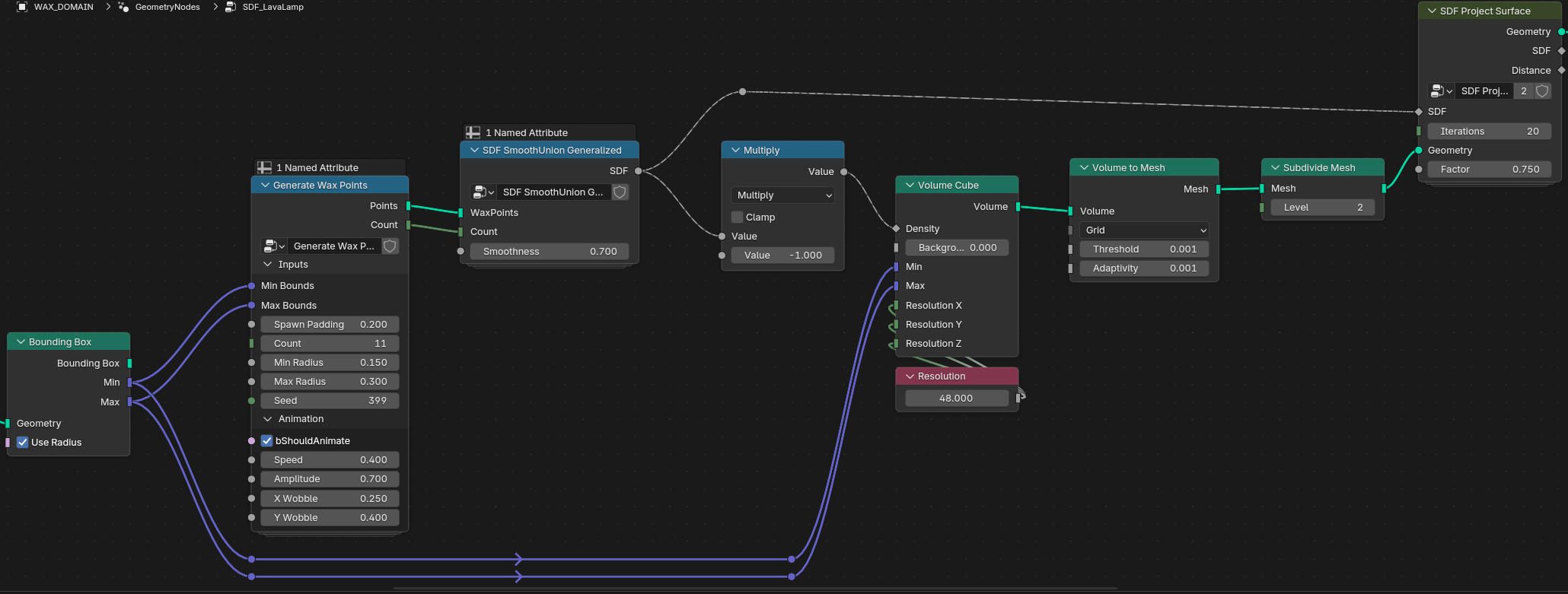
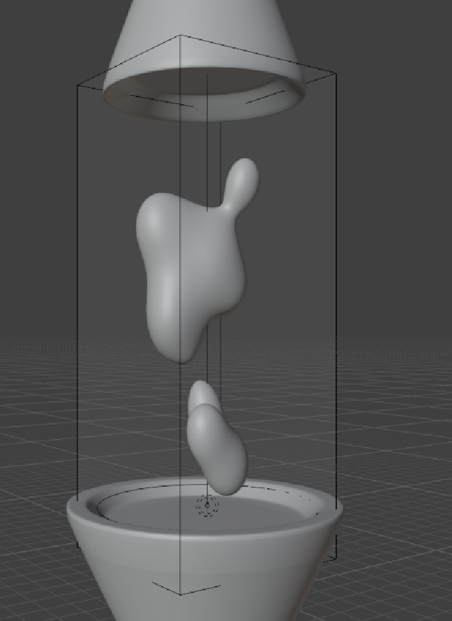
The same SDF is used in two places.

For the volume density I negate it:

\(\text{Density} = -\text{SDF}\)

This turns the inside of the SDF into the positive side of the scalar field expected by the volume meshing stage.

The original, non-negated SDF is kept around because it is needed again later for surface projection. (aka that last dark lime node on the far right of the last screenshot.)

Volume Cube and Volume to Mesh

#

Volume Cube samples the density field on a voxel grid between its Min and Max coordinates. In my graph, those coordinates come directly from the Bounding Box node of the source geometry, so the bounding box becomes the spatial domain of the SDF.

The bounding box is therefore more than an arbitrary container. It defines the spatial domain in which the SDF gets evaluated.

Volume to Mesh then extracts an initial isosurface from that sampled volume.

This already produces something recognizable, but it is still constrained by the voxel resolution. Increasing the resolution improves the result, although it also becomes increasingly expensive.

I also subdivide this first mesh before projecting it back onto the SDF. This gives the projection step more vertices to work with instead of trying to rescue a very coarse voxel mesh through mathematics alone. There are limits to my optimism.

I did not want resolution to be the only way of getting an accurate surface, so the next part of the setup refines the generated mesh against the original SDF.

Sampling the SDF Around a Mesh Point

#

For that refinement I first needed an estimate of the SDF gradient, so I made a small helper group called Mesh Capture SDF.

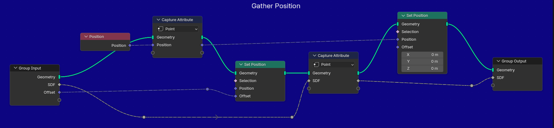
Its purpose is basically to answer this question:

What is the value of this SDF if I evaluate it at the same mesh point, but with a small positional offset?

The group:

1. Captures the original point position,
2. Temporarily offsets the mesh points by a small input vector,
3. Captures the SDF at the displaced location,
4. Restores the original position.

The geometry is therefore unchanged when it leaves the group. The useful result is the sampled SDF value.

This group is used four times in SDF to Mesh Normals.

Estimating the SDF Normal

#

SDF to Mesh Normals numerically estimates both a direction toward the surface and the local rate at which the SDF is changing.

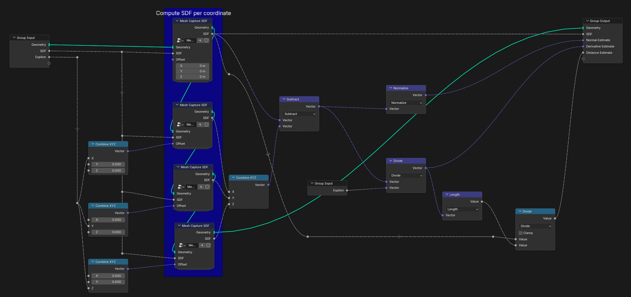
The group evaluates the SDF four times using Mesh Capture SDF: once at the current position, then once with a small positive offset along each coordinate axis.

If the current position is \(p\), the group samples:

\[ \Large \begin{aligned} d_0 &= d(p) \\ d_x​ &= d(p+(\epsilon,0,0)) \\ d_y​ &= d(p+(0,\epsilon,0)) \\ d_z​ &= d(p+(0,0,\epsilon)) \end{aligned} \]

where \(\epsilon\) is a small sampling distance.

Here there is one slightly non-obvious detail in the node graph.

The Subtract node is wired as the original sample minus the offset samples:

\[ \Large \Delta d = \begin{bmatrix} d_0-d_x\\ d_0-d_y\\ d_0-d_z \end{bmatrix} \]

A standard forward finite-difference gradient would normally use the opposite subtraction, while this vector that we have just created is an approximation of the negative gradient:

\[ \Large \dfrac{\Delta d}{\epsilon} \approx -\nabla d(p) \]

This is intentional and becomes useful in the projection step.

The non-divided vector is normalized to produce the Normal Estimate:

\[ \Large \hat{n} = \dfrac{\Delta d}{\lvert \lvert \Delta d \rvert \rvert} \]

Despite the node-group name (a bit of a misnomer on my part), this is actually pointing in the negative-gradient direction. With my SDF convention, that means roughly inward for a simple sphere.

The same vector is also divided by \(\epsilon\):

\[ \Large g_{\text{estimate}} = \dfrac{1}{\epsilon} \begin{bmatrix} d_x-d_0\\ d_y-d_0\\ d_z-d_0 \end{bmatrix} \]

This is what the node group outputs as Derivative Estimate.

The graph then calculates its length:

\[ \Large \lvert \lvert g_{\text{estimate}} \rvert \rvert \]

and uses that to obtain the Distance Estimate:

\[ \Large d_{estimate} = \dfrac{d_0}{\lvert \lvert g_{\text{estimate}} \rvert \rvert} \]

Why bother dividing by the derivative magnitude?

For a perfect signed distance function, the gradient magnitude is ideally 1 almost everywhere, so the raw SDF value already behaves like a distance.

After operations such as the smooth unions used for the wax, however, the resulting function is not guaranteed to remain a perfect distance function. Correcting by the locally estimated gradient magnitude gives me a more useful estimate for the projection step.

So, after all that math, the group gives me five outputs:

• Geometry
• SDF
• Normal Estimate
• Derivative Estimate
• Distance Estimate

And now I can finally use them to move vertices around. Maybe we’ll start seeing some results…

Projecting the Mesh Back Onto the SDF

#

The mesh produced by Volume to Mesh is only an approximation of the implicit surface. SDF Project Surface takes that mesh and iteratively nudges its vertices toward the SDF’s zero crossing.

Very warm thanks to Blender for implementing the “Repeat” node.

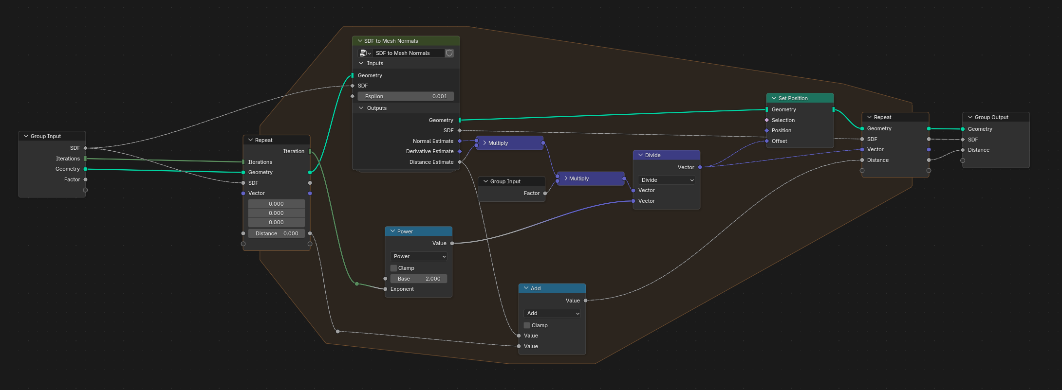
Inside the Repeat Zone, SDF to Mesh Normals is evaluated again on the current version of the geometry. This means every iteration gets a fresh normal and distance estimate after the previous correction has already moved the vertices.

The basic correction vector is:

\[ \Large \Delta p_i = \hat{n}_i \cdot d_{\mathrm{estimate},i} \cdot F \cdot \dfrac{1}{2^i} \]

Where:

• \(\hat{n}_i\) is the current Normal Estimate
• \(d_{\text{estimate},i}\) is the signed Distance Estimate
• \(F\) is the user-controlled projection Factor
• \(i\) is the current Repeat Zone iteration

The new point position is then simply:

\[ \Large p_{i+1}​=p_i​+\Delta p_i​ \]

The sign behavior is worth explaining because it looks slightly backwards at first.

Earlier, my Normal Estimate was built from the negative gradient. For a point outside the surface, the SDF is positive, so multiplying that inward-facing direction by a positive distance moves the point inward.

For a point inside the surface, the SDF is negative, so the same direction multiplied by a negative distance flips around and moves the point outward.

In both cases, the correction heads toward the zero surface.

The Factor lets me control how aggressively each step projects the mesh. On top of that, the correction is divided by:

\[ \Large 2^i \]

so each subsequent iteration becomes progressively smaller:

\[ \Large 1, \dfrac{1}{2}, \dfrac{1}{4}, \dfrac{1}{8}, ... \]

This damping makes the later passes more conservative instead of repeatedly firing vertices across the surface and hoping for the best.

The Repeat Zone also accumulates the Distance Estimate values through an Add node and carries the latest sampled SDF through to the output. The important output for the rest of the graph, though, is the projected geometry itself.

At this point I finally have a mesh that follows the implicit SDF much more closely than the first voxelized surface.

From Three Spheres to However Many I Feel Like

#

(or until my computer explodes)

The first working version of this setup was not particularly procedural.

I had three SDF Sphere groups.

Then I had two SDF Smooth Union groups.

And if I wanted a fourth blob, I could lovingly copy and paste another pair of nodes until the graph became a crime scene.

Not really scalable, is it?

What I really wanted was:

1. Generate an arbitrary number of blob centers.
2. Give every blob its own radius.
3. Evaluate an SDF Sphere from that data.
4. Smooth-union all of them together.
5. Keep the rest of the meshing pipeline completely unaware of how many blobs exist.

This became two node groups: Generate Wax Points and SDF SmoothUnion Generalized.

Generating the wax points

#

Generating the Wax Points

Generate Wax Points creates the lightweight data that represents the wax before any SDF is actually evaluated.

I start with a Mesh Line, using its Count simply as a convenient way of generating an arbitrary number of indexed points.

Technically, Mesh Line also gives me edges. I do not care about them. Later code only samples data from the point domain, so the vertices are the useful part.

Each point represents one future wax blob.

A Random Value in Vector mode chooses its initial position between the padded minimum and maximum bounds, using the point Index as its ID.

Another Random Value, this time a Float, chooses the blob radius between Min Radius and Max Radius.

That value is stored on every point as a named float attribute:

wax_radius

The result is a tiny procedural description of all the wax:

point position = blob center
wax_radius     = blob radius

No visible sphere geometry needs to be instantiated.

That turns out to be extremely convenient, because I can move these points around later and let the SDF system worry about rebuilding the actual shape.

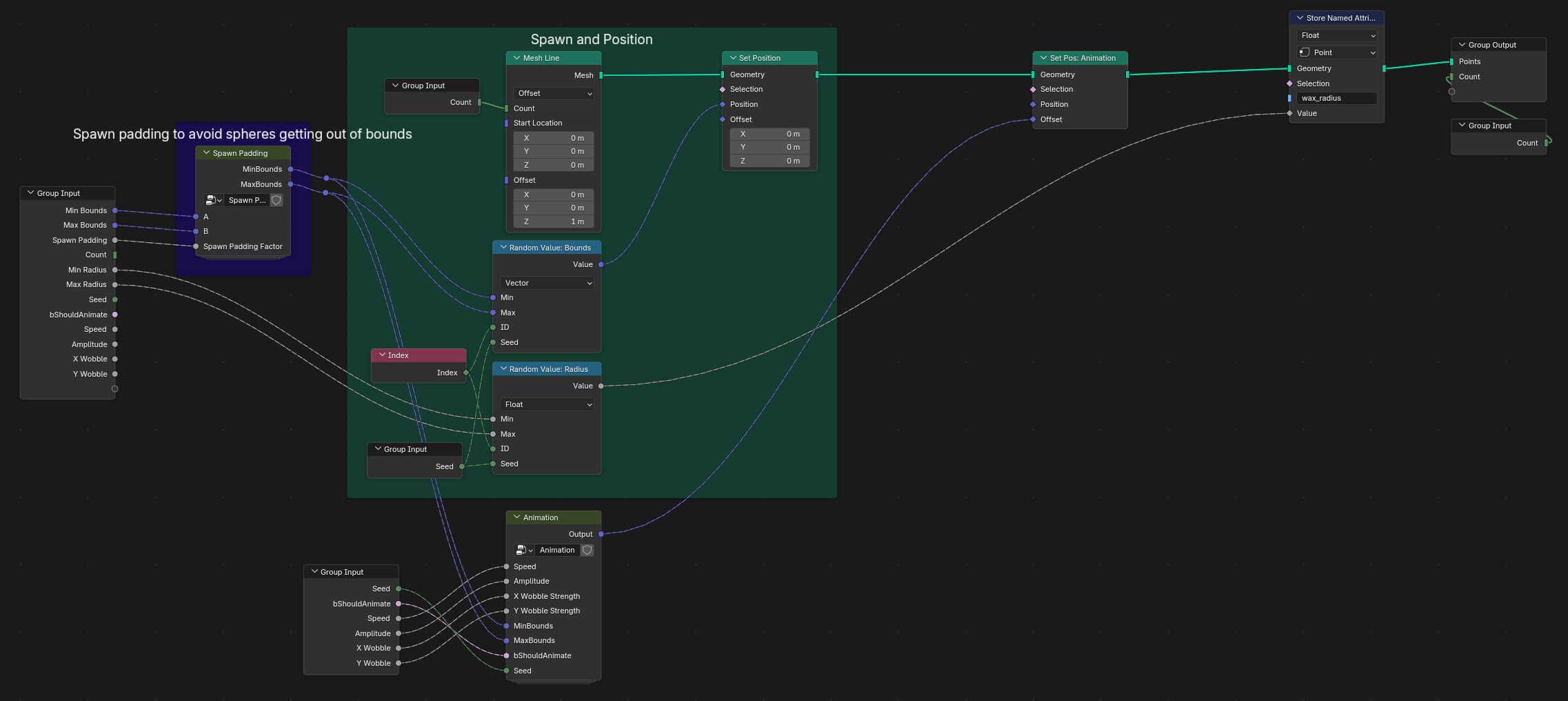
There’s extra work in here, but I’m going to elaborate on the important bits only. This article is getting lengthy.

Generalizing the smooth union

#

Now I have an arbitrary number of points, but SDF Smooth Union still only accepts two SDFs at a time.

Enter another Repeat Zone.

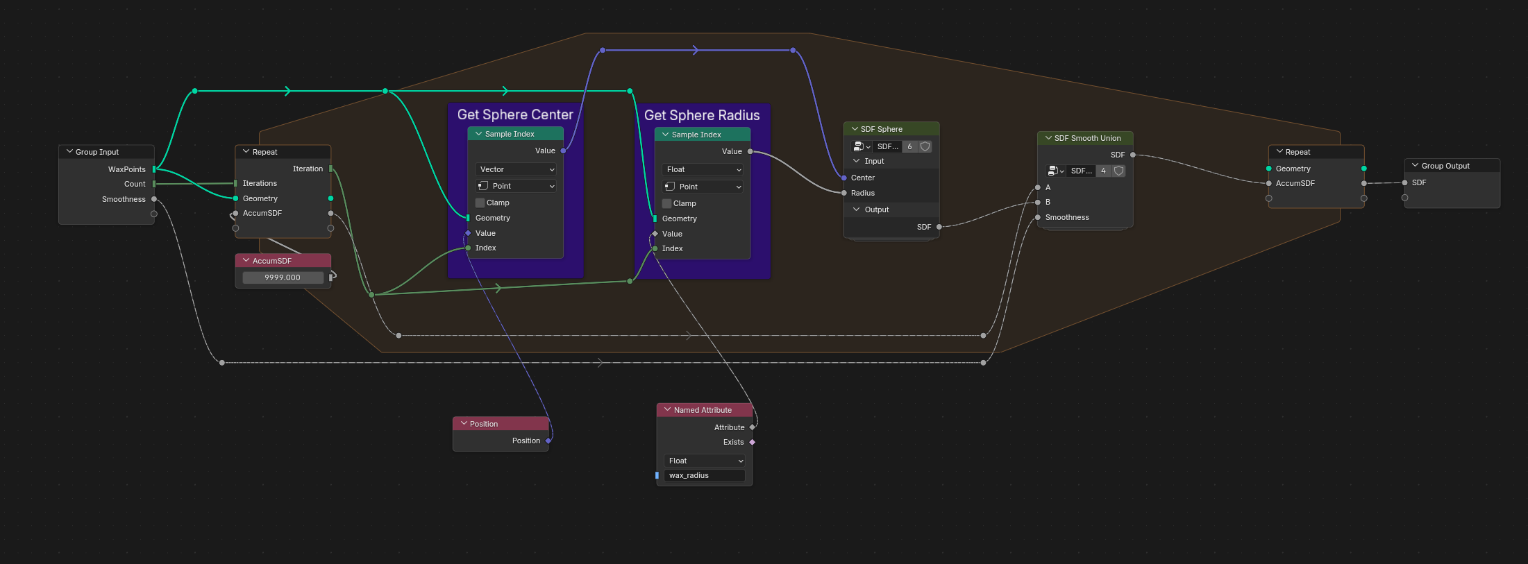
The loop runs once for every wax point.

I initialize an accumulated SDF to: \(9999\) (not pictured here), think of it as a very large number that will be surely overwritten.

For each iteration, two Sample Index nodes read the current point.

One samples its position:

$$ c_i = Position[i] $$

and the other samples the wax_radius attribute:

$$ r_i = wax\_radius[i] $$

Those two values are passed into the same SDF Sphere group from the beginning of the article:

$$ d_i(p)=\lVert p-c_i\rVert-r_i $$

The resulting sphere SDF is then combined with the value accumulated by all previous iterations:

$$ D_{i+1} = SmoothUnion(D_i,d_i,k) $$

After Count iterations, the group outputs a single SDF representing every wax blob. Amazing. We gotta move them now.

Making the Wax Move

#

At this point I had procedural blobs, but they were displaying the dynamic behavior of decorative rocks.

Fortunately, the way the system is structured makes animation fairly painless.

I do not animate the final mesh.

I animate the wax points inside Generate Wax Points, before their positions are sampled by the generalized SDF union.

The Animation group splits the movement into three smaller groups:

AnimateZ, which provides the main vertical movement AnimateX, an optional horizontal wobble AnimateY, another optional horizontal wobble

Their outputs are combined into one XYZ offset and passed into the second Set Position node inside Generate Wax Points.

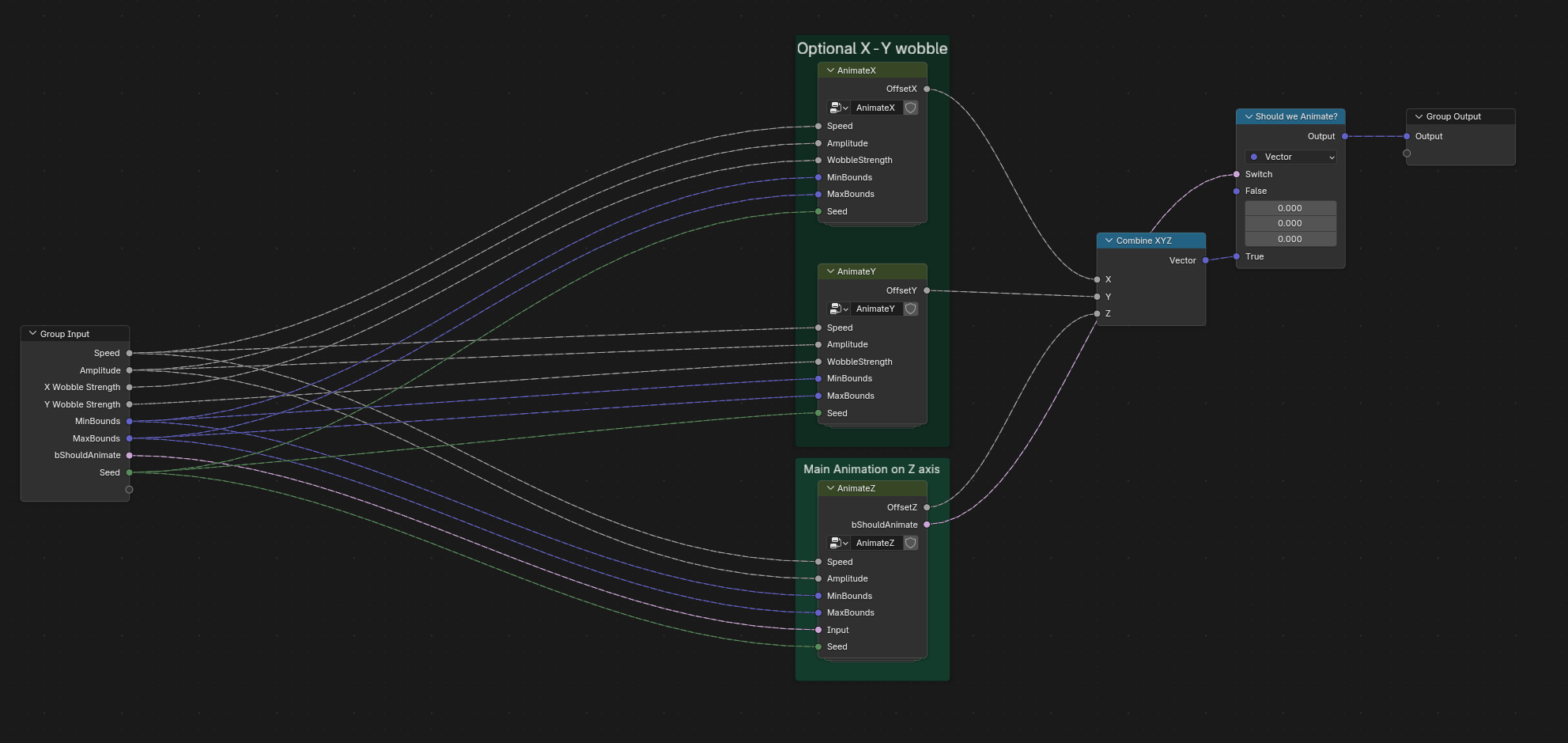
I won’t elaborate much on the math here, what’s happening behind the scenes is the basics of procedural animation: sine and cosine waves, and modulating their amplitude, frequency and phase as I see fit (or as the rand nodes see fit, rather).

Here’s what the first working prototype finally looked like:

Pretty nice, I think we’re at a good spot, finally!

Putting Everything Together

#

At the top level, the finished wax graph is surprisingly compact compared to the questionable decisions hidden inside its node groups.

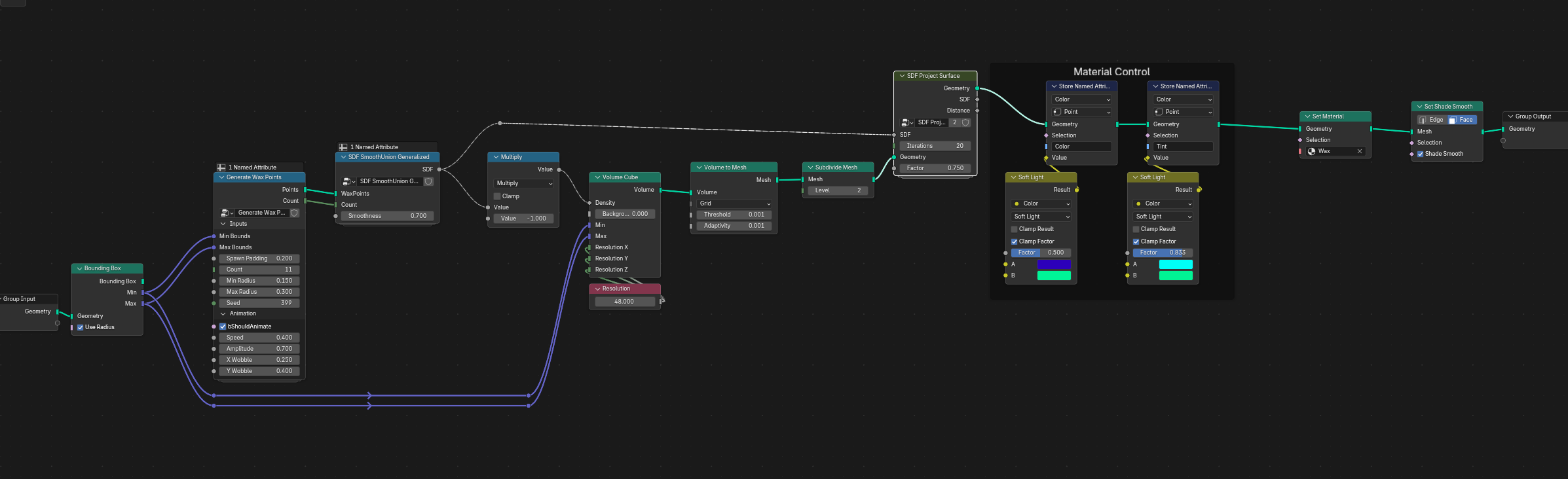
The complete pipeline is, in case you’re having trouble reading:

Input ->
    -> Bounding Box
    -> Generate Wax Points
    -> SDF SmoothUnion Generalized
    -> Negate SDF
    -> Volume Cube
    -> Volume to Mesh
    -> Subdivide Mesh
    -> SDF Project Surface
    -> Material Attributes
    -> Set Material
    -> Shade Smooth
        -> Output

I’ll gloss over the lava lamp modelling, and the tricks to visually render water and glass, as it’s mostly smoke and mirrors that I grabbed from previous knowledge and online tutorials.

Here is the final result!

Final thoughts and Possible Extensions

#

There are a few directions in which I could take the system further.

A temperature model would be the obvious one. Instead of oscillating around fixed spawn positions, blobs near the bottom could accumulate “heat”, gain upward velocity, cool near the top, and eventually sink again.

The bounding volume could also become an actual lamp-shaped SDF rather than a generic box. That would allow the wax field itself to be constrained against the interior glass shape.

Radius could vary over time, allowing blobs to stretch or shrink slightly during their vertical cycle.

The spawn padding could become radius-aware, guaranteeing that every initial sphere fits inside the valid region.

There is also plenty of room for better motion. The current sine-based approach works because the smooth union does a lot of visual work for free, but slower noise, stateful motion, or Simulation Zones could produce much less periodic trajectories.

For now I prefer the current version because it remains (mostly) readable. Every major part of the effect can still be followed from the node graph without turning it into a miniature physics engine.

Thank you for reading! This was an hard write-up, taking a lot of hours. If you find any errors or mistakes, please let me know.